


When a subscriber receives a campaign text, clicks, and then completes a purchase, how much of that purchase did the campaign cause? And when someone opts out right after a send, was it the campaign or something else? Answering either question requires the same thing we needed for journeys: what the same subscribers would have done if the campaign had never been sent.
In our previous post, How Attentive Measures Incrementality, we measured the incremental effect of journey messages – the texts that fire automatically when a shopper abandons a cart or a browsing session. There, a quiet-hours cutoff created a natural experiment: shoppers minutes apart landed on different sides of a rule they couldn’t see.
Campaigns work differently. A marketer chooses the message, the audience, and the send time, and the whole audience receives the text at roughly the same moment. There is no cutoff to exploit, and the subscribers who receive a campaign were picked on purpose. Measuring what a campaign causes therefore needs a different design – one built around time rather than a threshold.
The question, though, is the same. The value of a campaign isn’t the purchases that follow it. It’s the difference between what happened after the send and what would have happened without it: the counterfactual. The same logic applies to opt-outs. Some subscribers would have opted out that day anyway, and we should only assign an opt-out to a campaign if the campaign caused it.
The simplest approach is to compare recipients’ behavior in the hour before a campaign with the hour after it. If purchases go up, credit the campaign. The problem is that many other things change around a send. Shopping follows the clock: activity rises through the morning, peaks around lunch and in the evening, and shifts with the day of the week. A brand may launch a sale on the same day, or the whole market may be busier because of a holiday. A before-and-after comparison mixes the campaign’s effect with all of these.
The opposite approach – comparing recipients with subscribers who didn’t receive the campaign, after the send – has the reverse problem. Marketers choose campaign audiences deliberately, often targeting subscribers who are more engaged or more likely to buy. Recipients might convert at higher rates even if the campaign did nothing.
Attribution inherits a version of both problems. It records conversions that follow a campaign within a fixed window, so it can credit a campaign for purchases that recipients would have made anyway. And it has no natural way to tell whether an opt-out came from the message itself or from something else that happened that day.
The difference-in-differences (DiD) design combines the two flawed comparisons into one that addresses both problems under a single assumption. Instead of comparing levels, it compares changes: how much did recipients’ behavior change from before to after the send, compared with how much the control group’s behavior changed over the same window?
The control group’s change captures what would have happened anyway, as long as it affects both groups alike – the time of day, the day of the week, the brand’s sale. Subtracting it from the recipients’ change leaves the part of the change that only recipients experienced: the campaign, together with anything that reaches recipients because of it, such as journeys the campaign triggers or an email sent to the same audience.
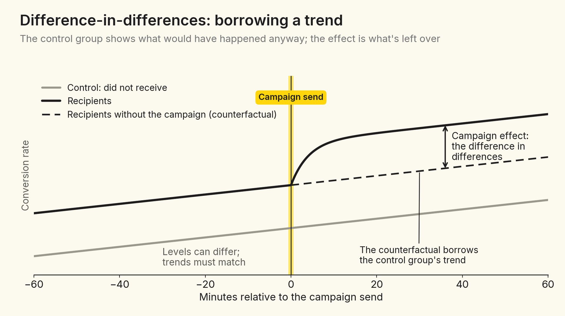
Imagine that in the hour before a send, 20 of every 10,000 subscribers in both groups make a purchase. In the hour after, 50 of every 10,000 recipients buy, but so do 30 of every 10,000 subscribers who didn’t receive the campaign – an evening uptick that has nothing to do with the message. A before-and-after comparison would credit the campaign with 30 purchases per 10,000 recipients. The difference-in-differences credits it with 20: the recipients’ increase of 30 minus the control group’s increase of 10.
DiD=(recipients after−before)−(control after−before)
The two groups don’t need to start at the same level. If recipients were more active to begin with, that gap appears both before and after the send and cancels out. What the design needs is that the two groups would have changed in the same way without the campaign. That’s a statement about changes in levels, so it’s most credible when the groups start at similar levels; with very different baselines, a proportional evening uptick alone would open a gap.
That requirement is called the parallel trends assumption: absent the campaign, the outcomes of recipients and control subscribers would have evolved in parallel. If it holds, any divergence between the two groups after the send can be attributed to the campaign.
Like every counterfactual, the assumption can’t be tested directly – we never observe recipients in the world where the campaign wasn’t sent. But it has a testable implication. If the two groups would have moved together after the send, they should also have moved together before it, when nothing had yet happened to pull them apart. A flat pattern of pre-send differences – small next to the post-send effects, and tested jointly rather than bin by bin – is evidence that the design is doing its job; a sloped pattern is a warning sign that the groups were never comparable to begin with. With samples this large, almost any difference is statistically significant, so size matters more than significance.
Clean pre-trends are the minimum condition for a causal reading, not a guarantee. Marketers select campaign audiences on purpose, sometimes based on behavior far back in time, and parallel trends in the hour before a send can’t rule out every form of selection. For the targeting levers we discuss later, that selection is both a concern and the very thing we want to learn about.
For each campaign, we split the brand’s reachable subscribers into three mutually exclusive groups:1
Comparing these groups in pairs answers three different questions.
Three groups, three comparisonsFor every campaign, we follow the brand's reachable subscribers in three groups and compare them in pairsBCNo-click vs. control: hownon-clickers change after the sendClicked vs. no-click: howclickers differ from non-clickersDid not receivecontrolReceived, did not clickreceived-no-clickReceived and clickedreceived-and-clickedAClicked vs. control: how subscribers who engage with the campaign changeClicking is a choice made after the send. Only all recipients vs. control compares groups fixed before it
Figure 3. The three groups we follow for every campaign, and the question each comparison answers.
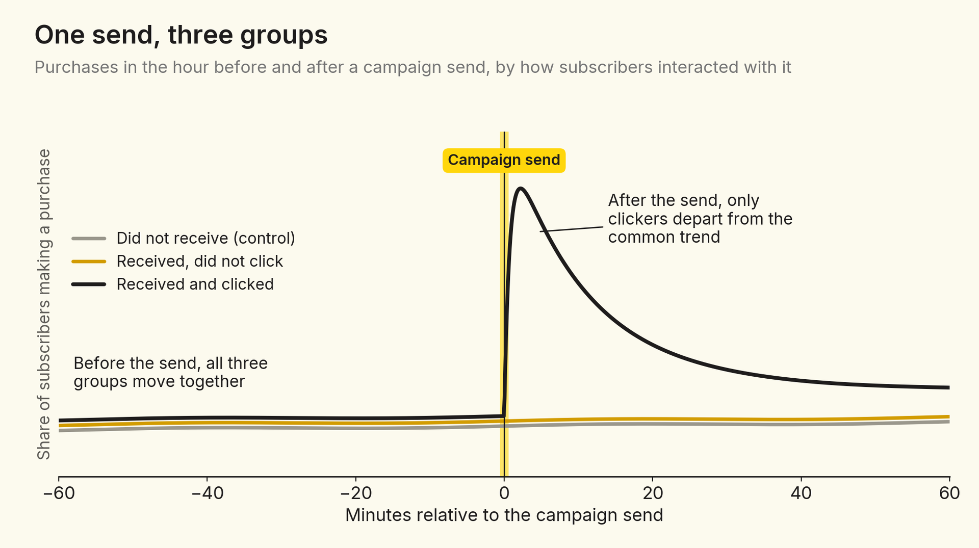
Clickers versus control measures how the behavior of subscribers who engage with the campaign changes relative to subscribers who never received it, across site visits, product browsing, cart additions, purchases, and opt-outs. Received-no-click versus control compares how recipients who don’t click change relative to the same control. And clickers versus received-no-click compares subscribers who all saw the same message at the same moment but made different choices about it. Because clicking is a choice made after the send, these comparisons describe groups defined by that choice; only all recipients versus control compares groups fixed before the send.
The middle comparison does double duty. For shopping outcomes, it’s a first check on selection: if subscribers who receive the campaign but don’t click show no lift, the effect we see among clickers is less likely to come from the campaign’s audience simply being on a different trajectory. For opt-outs, it speaks to a substantive question – whether unsubscribes come from engaging with the content or from the send itself – which matters for how marketers should target.
Campaigns go out on different days, at different hours, for different brands. To pool them, we put every campaign on its own clock: minute zero is the moment the campaign’s first message arrived, and everything is measured in minutes, hours, or days relative to that send. A campaign sent on a Tuesday morning in March and one sent on Black Friday both start at zero.2
Lining up campaigns on event timeCampaigns go out on different days and at different hours. Each one gets its own clock, starting at its sendCalendar timeJanFebMarAprMayJunJulAugSepOctNovDecTue, Mar 410:00amWed, Jun 182:30pmTue, Sep 97:15pmFri, Nov 289:00amalign every campaign on its own sendEvent timeTue, Mar 4, 10:00amWed, Jun 18, 2:30pmTue, Sep 9, 7:15pmFri, Nov 28, 9:00am-60-40-200204060Minutes relative to each campaign's own send
Figure 4. Campaigns sent on different dates and at different times of day are aligned on their own send times, so every campaign starts at minute zero.
Within event time, we split the hours and days around the send into short bins – five minutes wide in the first hour – and estimate the same simple regression for each outcome, each pair of groups, and each bin:
Outcome=α+β·Post+γ·Group+δ·(Post×Group)+ε
Here, Post marks the bin being estimated as opposed to the reference period, Group marks the treated group in the pair (for example, clickers rather than control), and δ – the coefficient on their interaction – is the difference-in-differences estimate for that bin. Three design choices matter:
Plotting the bin-by-bin estimates gives the classic event-study picture. Before the send, the estimates should hover around zero; after the send, any effect shows up as a departure from zero. In our data, all three groups follow almost exactly the same path in the hour leading up to a send across site visits, product browsing, cart additions, purchases, and opt-outs.
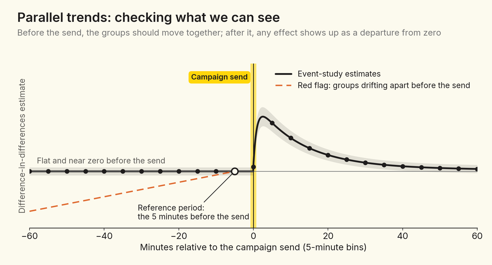
We don’t see a meaningful pre-trend: pre-send differences are negligible next to the post-send effects. If we did, the econometrics literature offers ways to deal with it: explicitly modeling the trend in the regression, for example with a group-specific time trend, or applying one of the recently proposed corrections for event-study designs, which bound the post-send deviation using the pre-send one or use additional variables that track the confounder.4 These fixes come at a price, though.
First, they leave an important question outside the estimate itself: what mechanism created the pre-trend, and what kind of selection is it? For us, that’s not a nuisance to be adjusted away. Audience targeting is one of the questions we care about most, and a pre-trend would be a direct signal about how campaign audiences are chosen.
Second, they go to the heart of the design’s assumptions. Parallel pre-trends are only a suggestive indicator of parallel post-trends – the assumption that actually matters. Mechanically “fixing” a pre-trend gives little assurance about the counterfactual post-trend, and it requires an additional assumption: that the selection process behind the pre-trend is stable, and would have kept shaping recipients’ behavior after the send in the same way it did before.
Clicking is a choice that subscribers make after the message arrives, so clickers are not a random slice of recipients. Perhaps subscribers who were about to shop anyway are simply more likely to click. Two pieces of evidence speak to that concern. First, clickers’ behavior before the send looks the same as everyone else’s; if they were already on their way to the store, it would show up in the pre-period. Second, recipients who don’t click show no meaningful lift in purchases per subscriber.
Neither piece of evidence is conclusive. A subscriber who happens to be in a shopping mood at the very moment the message arrives may both click and buy, and nothing in the pre-period would reveal it. And because only a small share of recipients click, even slight negative selection among non-clickers would correspond to strong positive selection among clickers.
The comparison that doesn’t depend on who chooses to click is all recipients versus control. Its effect is the click rate times the effect among clickers, plus the share of non-clickers times the effect among non-clickers. That gives us a cross-check: if the campaign does nothing for subscribers who don’t click, the effect per click should equal the effect on all recipients divided by the click rate – the same ratio logic as the LATE in our previous post. When the two agree, selection into clicking is less likely to be driving the clicker estimates.
For the same reason, we read the clicker comparison as the effect of a campaign for subscribers who choose to engage with it, not as the effect of a click on a random subscriber. And for site visits and browsing, part of the clicker effect is mechanical – a click on a link is itself a site visit – which is why purchases and opt-outs are the outcomes that matter most.
The three-way comparison tells a different story for opt-outs. Opt-outs rise among recipients who didn’t click by a large share of what clickers show. Because non-clickers are nearly everyone, most incremental opt-outs come from the send itself rather than from engaging with the content. For marketers, that points toward targeting subscribers who are likely to click and making campaigns more clickable, rather than sending more broadly.
Bin-by-bin estimates answer a question about timing. Each pointwise estimate measures the extra share of a group that experiences an outcome within a bin – for example, the extra share of clickers who purchase between minutes 15 and 20 after the send. The pointwise series shows when the behavior happens, and it’s the series the pre-trend check looks at.
For decisions, the more useful number is usually the total. A cumulative estimate measures the extra share of a group that has experienced the outcome at least once by a given time since the send – for example, the extra share of clickers who have made at least one purchase by the end of the first day.
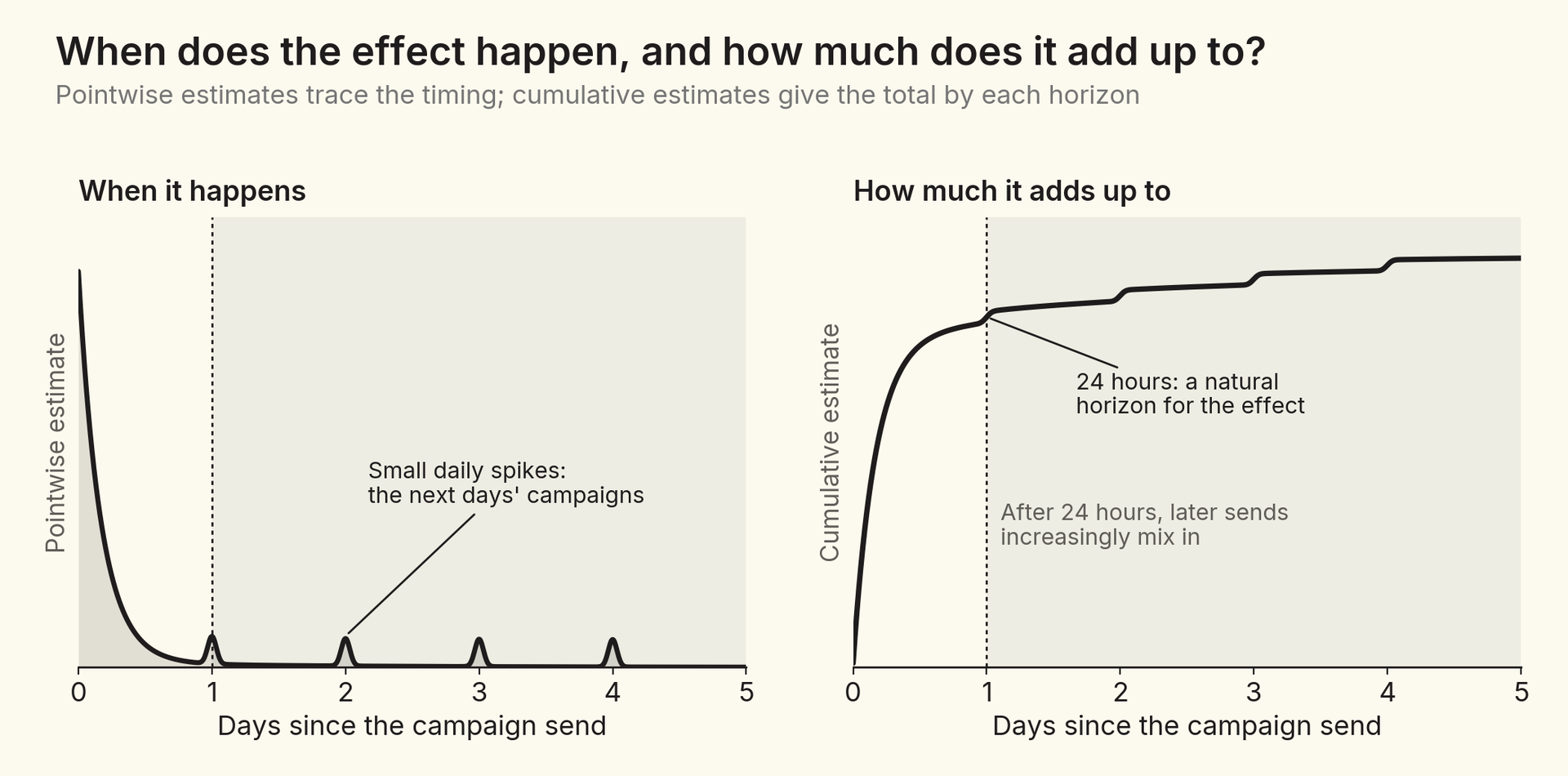
Longer horizons bring a practical complication. Brands send campaigns regularly, and subscribers who received today’s campaign are also more likely to receive tomorrow’s. In the pointwise estimates, this shows up as small spikes every 24 hours after the original send. Those spikes mark the point where the clean comparison starts to blur, which makes the 24-hour mark a natural horizon for reading causal effects. Longer horizons are still informative, but they increasingly measure today’s campaign together with the later sends that tend to follow it.
There are two natural ways to pool thousands of campaigns. In the unweighted version, each campaign counts as one observation in every cell, regardless of its audience size, so the estimate describes the average campaign and the largest senders don’t mechanically dominate. In the weighted version, each campaign counts in proportion to its audience, so the estimate describes the average subscriber. Neither is “right” – they answer different questions.

When effects are similar across campaigns, the two estimates agree. When they differ, the gap itself is informative: it tells us that effects vary with campaign size. Comparing the two for conversions and opt-outs separately shows whether smaller and larger campaigns get the same exchange of purchases for unsubscribes, and when in the life of a campaign any difference opens up. Campaign size isn’t just brand size, though: targeted campaigns are smaller by design, so a gap between the two can reflect targeting as much as scale.
The same machinery can evaluate campaign levers: targeting a segment instead of sending to everyone, bypassing fatigue rules, winning back subscribers who didn’t click a previous campaign, retargeting subscribers who clicked but didn’t purchase, or reaching low-propensity shoppers.
Every lever like this delivers two treatments at once: the campaign message itself, and the selection of the audience that receives it. What we measure is the combination of the two, and we want to disentangle them – not because one part is good and the other bad, but because each is something a marketer can improve.
For us, selection is an important, good part of the effect. The difference-in-differences design already removes one bad kind: stable differences in how likely subscribers were to buy anyway. As long as the audiences would also have trended alike, what remains when we compare them is closer to what economists call selection on gains – careful targeting picks subscribers who respond more to the message.5 Part of a campaign’s effect comes from that targeting, and that part can be improved too. Parallel trends deserve the most care for segments chosen on recent behavior, such as retargeting and win-back audiences, whose activity may already be rising or fading on its own.
Disentangling the two treatments takes care. Campaigns that use a lever are chosen deliberately, and they may differ from other campaigns in ways that have nothing to do with whom they target: a stronger offer, a more engaged brand, a better-timed send. To separate the audience from the campaign, we look through three lenses. The second and third apply when a campaign’s recipients include both subscribers picked by the segment and others, as when a retargeting or win-back segment is added to a broader send:
Is it the audience or the campaign?Three lenses for evaluating a targeting lever, from the broadest comparison to the most controlled1Between campaignsUses the leverOther campaignsvs.Campaigns that use the lever vs. othercampaigns. The headline comparison, but itmixes the lever with everything else thatdiffers about these campaigns.2The untargeted audienceUses the leverOther campaignsvs.Recipients of lever campaigns who weren'ttargeted vs. other campaigns. If they alsodo better, the difference is about thecampaign, not the audience.3Within the campaignUses the levertargetednottargetedTargeted vs. non-targeted recipients of thesame campaign. Same message, brand, andsend time, so differences reflect the audience.selected by the lever's segmentother recipientsoutlined: the subscribers comparedbroader: more campaigns, more room for other differencesmore controlled: the same campaign
Figure 8. Three lenses for evaluating a targeting lever, from the broadest comparison to the most controlled.
When the three lenses agree, we can be more confident about how much of a lever’s effect comes from whom it targets and how much from the campaign itself. When they disagree, they tell us where to look next – and often point toward a randomized test.
One caution applies to all three lenses. A lever can change who clicks as well as how much each click is worth. A lever that brings in many marginal clickers may lower the average effect per click while raising the campaign’s total effect, so we look at click rates alongside effects per click rather than comparing per-click effects alone.
Campaigns don’t come with a convenient cutoff, but they do come with a precise clock. An event study uses that clock: by lining up thousands of campaigns on their own send times and comparing how recipients and non-recipients change around each send, it separates a campaign’s effect from the rhythms of the day, the week, and the market.
Three groups instead of two turn a single estimate into a richer picture: the causal effect on all recipients, and how it divides between subscribers who click and those who don’t. Pointwise and cumulative estimates show when effects happen and how much they add up to, weighting shows whether they differ by campaign size, and three lenses help separate the two treatments every campaign delivers – the message and the audience it reaches.
The design has limits. It relies on parallel trends, which we can support but never prove, and on a horizon short enough that later sends don’t blur the comparison. Where the lenses disagree, the right next step is a randomized test. But for the everyday question of what a campaign caused, event studies let us answer it at scale, across thousands of campaigns, without holding back messages from anyone.


