


When a shopper abandons a cart, receives a text, and then completes the purchase, how much of that purchase did the text cause? Answering this requires something we can never observe directly: what the same shopper would have done if the text had never been sent.
Every triggered message is a small intervention. A shopper leaves a cart or a browsing session behind, and a few minutes later the brand reaches out. If the shopper comes back and buys, it's tempting to give the message the credit. But the shopper might have come back regardless: the cart was already full and the decision half made. The value of the message isn't the purchase itself. It's the difference between what happened with the received message and what would have happened without the message.
Economists call that difference a causal, or incremental, effect, and the scenario it's measured against a counterfactual.
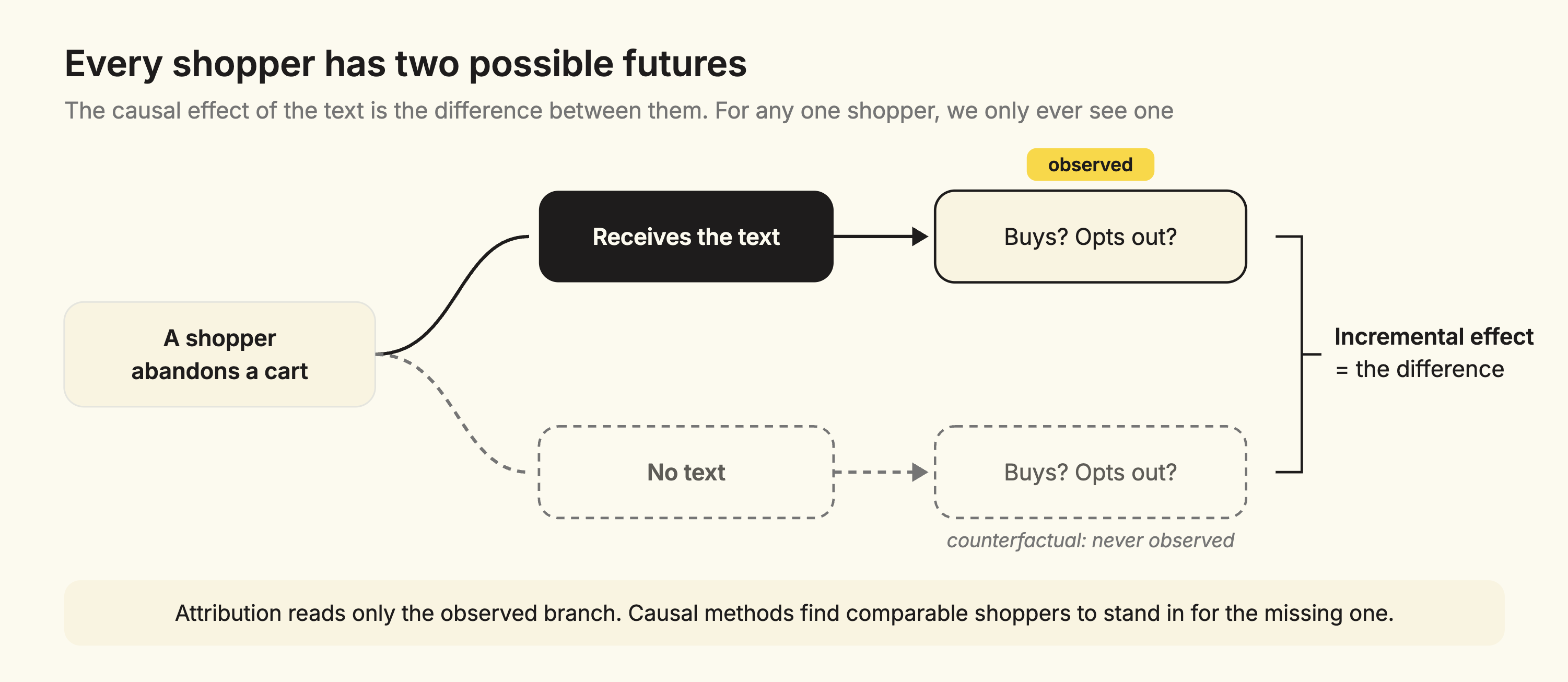
The same logic applies to opt-outs. Some shoppers opt out of SMS after receiving a message. Others would have opted out anyway, because of a different message, a change of heart, or simply a crowded inbox. We should assign an opt-out to a journey text only if this message caused the opt-out.
Incremental conversions and incremental opt-outs are the key quantities we need to decide how many journey texts to send, to whom, and how strongly fatigue rules should hold them back.
Attribution often answers a different question. It records which conversions and opt-outs followed a message within some window. That describes what happened after the message, not what happened because of it.
The gap between the two is selection bias. Marketing journeys are triggered by intent: shoppers enter them precisely because they were close to buying. Shoppers who receive these messages would convert at higher rates even if the messages did nothing, and attribution may fold that baseline intent into the message's credit. On the opt-out side, something like a last-touch rule would assign each opt-out to whichever message arrived last, whether or not that message was the reason behind the opt-out.
These selection biases don't have to point in the same direction. Attribution can overstate a message's effect on conversions, understate it when conversions the message did cause get credited elsewhere, or misplace opt-outs across journeys. Without observing a counterfactual world where the journey message did not arrive, there's no way to know which way the error runs, or how large it is.
One of the standard ways to get a counterfactual is a randomized experiment. If a coin flip decides who receives the journey message and who does not, the two groups, when large enough, end up alike in every respect except the message: intent, purchase history, cart value, and everything we can't measure. The average outcome of the holdout group then becomes a credible stand-in for the average outcome in the missing future of the treated group.
Randomized holdouts are costly in practice. They withhold messages, and therefore revenue, from real shoppers, and they need time to collect enough data, journey by journey. What we wanted at Attentive was the comparability of a randomized experiment without having to run one.
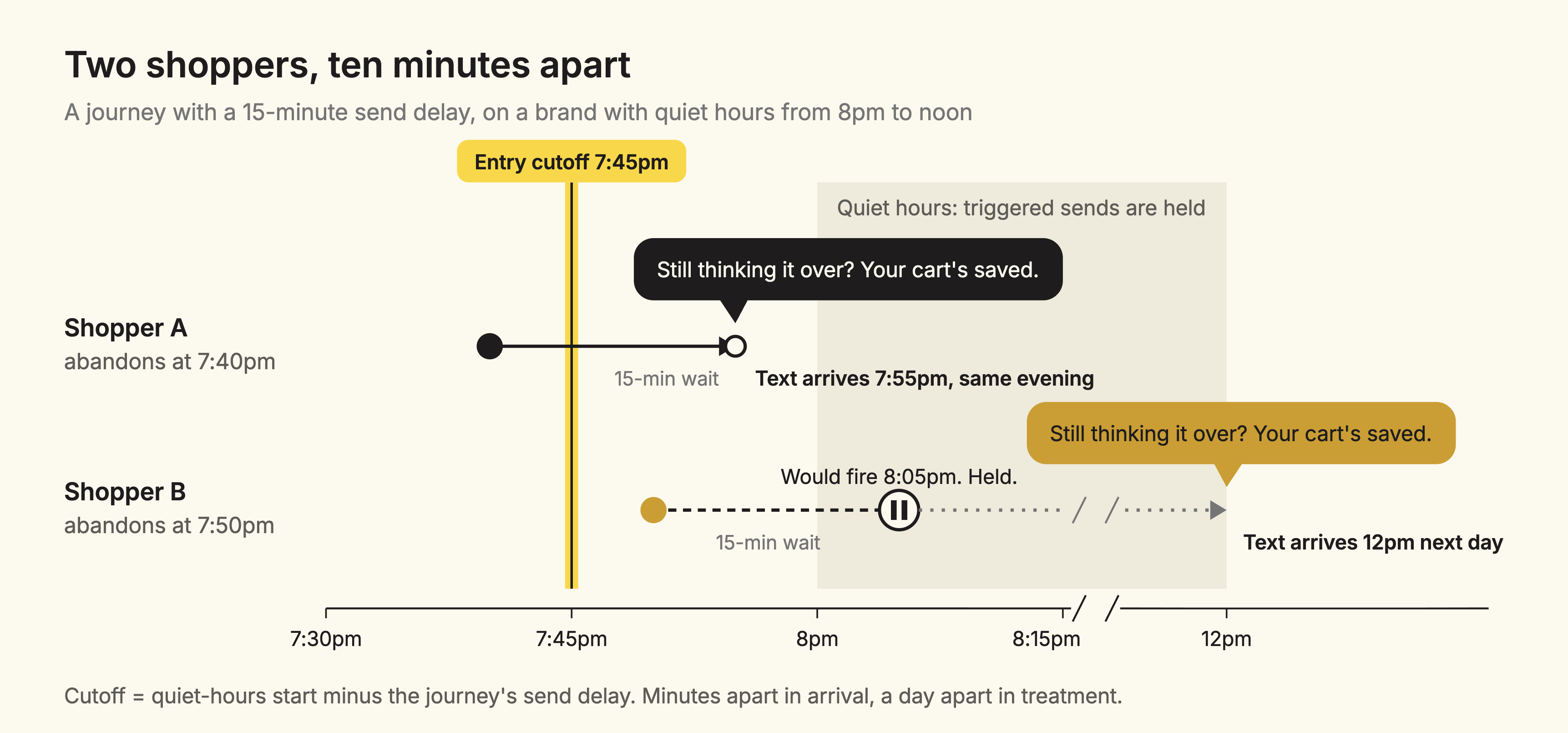
Most brands pause SMS sending overnight. A common setting holds any triggered message that would fire between 8pm and noon until the sending window reopens the following day.1
Combine that rule with a journey's send delay, and you get a sharp cutoff in time. A journey that waits 15 minutes before its first message can send it the same evening only if the shopper enters before 7:45pm. A shopper who enters at 7:40pm gets the text at 7:55pm. A shopper who enters at 7:50pm would get it at 8:05pm, inside quiet hours, so it waits until noon the next day, long after the moment of intent has passed.
For practical purposes, those two shoppers are the same kind of shopper. They were browsing on the same evening, minutes apart. Neither knows or considers, when shopping, the brand's quiet hours or the journey's delay, so neither could have realistically chosen which side of the cutoff to land on. The rule, not the shopper, decides who gets an evening text.
This is what economists call a natural experiment: a situation in which some mechanism or a rule outside people's control assigns treatment in a way that is as good as random.
We measure each shopper's entry time relative to their own journey's cutoff, defined as the quiet-hours start minus the send delay. That re-centering allows us to pool brands with different quiet windows and journeys with different delays into a single design. For every journey, minute zero is the last moment an evening text is still possible.
A regression discontinuity design (RDD) applies whenever a rule assigns treatment based on whether a continuous measure, called the running variable, falls above or below a threshold. Classic examples include scholarships awarded above a test-score cutoff, or social security programs available below an income threshold. The key assumption for RDD is continuity: everything about people that affects their outcomes changes smoothly along the running variable, and only the treatment rule changes abruptly at the cutoff. This means that if outcomes jump at the cutoff, the rule is the only thing left to explain that jump.
Intuitively, a shopper who enters at 7:44pm and one who enters at 7:46pm are about as similar as two shoppers can be. Any systematic difference in what they do next, beyond what a smooth trend over the evening would produce, has to come from the one thing that changed between them: whether the journey text arrived that evening.
The price of this credibility is that the comparison is local. We learn about shoppers near the cutoff, in the evening, whose journeys were eligible to send. We'll come back to what that means for the bigger picture later.
In a textbook RDD, crossing the cutoff switches treatment fully on or off. Ours doesn't. Crossing the cutoff makes an evening text far less likely, but not impossible. Some shoppers after the cutoff still receive an SMS overnight, because of time zone differences, brand-specific settings, or marketing software setup. And some shoppers before the cutoff receive no text at all, because fatigue rules or frequency caps suppress it.
When a cutoff shifts the probability of treatment rather than determining it in 0/1 fashion, the design is called a fuzzy regression discontinuity.
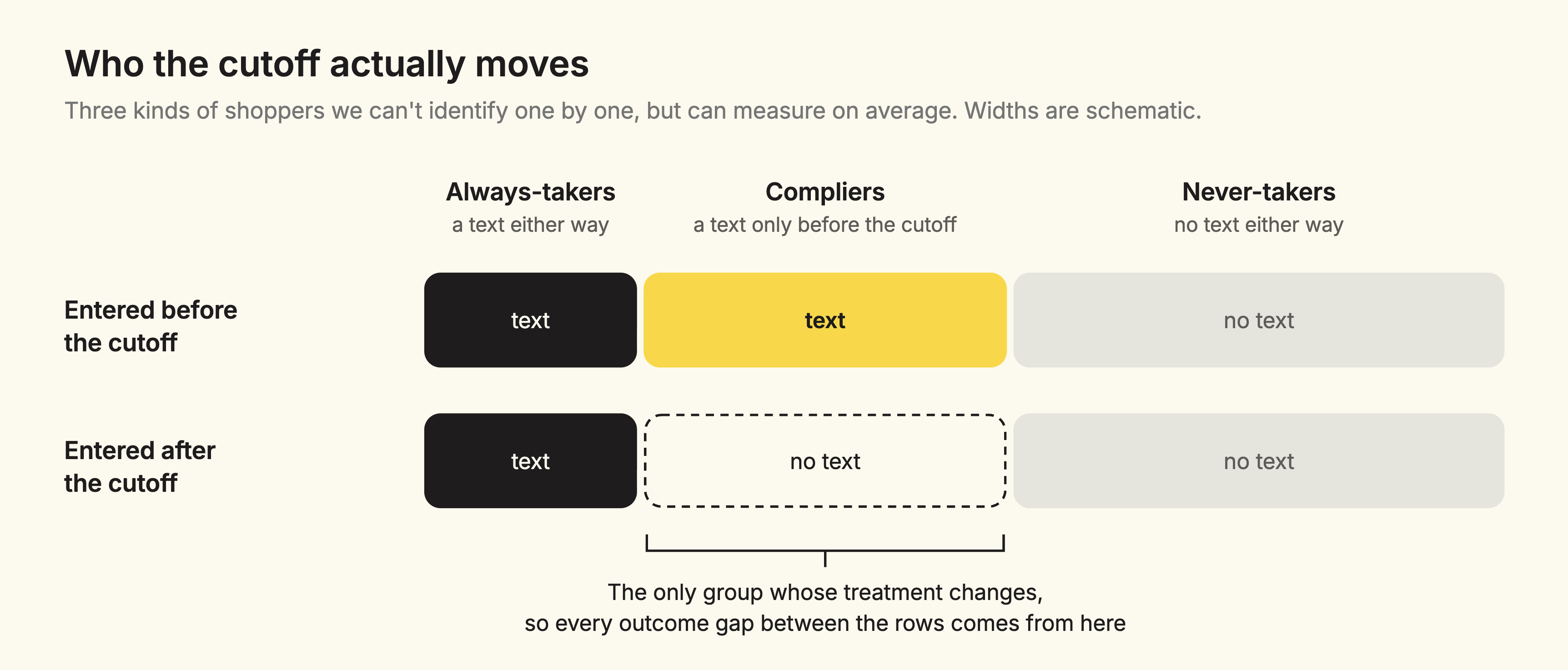
The fuzzy design also gives us a useful way to think about whom we learn from. Relative to the cutoff, every shopper falls into one of three groups:
Because the cutoff changes nothing for always-takers and never-takers, it can only change outcomes through compliers. That's the logic that turns a comparison of two crowds into the effect of the message itself.2
Unfortunately, we can’t tell to which of the three groups shoppers belong since we can observe each shopper only in one of the worlds – entering the journey before or after the cutoff – but to classify them we need to know whether a shopper received a journey text in both worlds. However, with causal methodologies we can tell something about the average effects on these shopper groups.
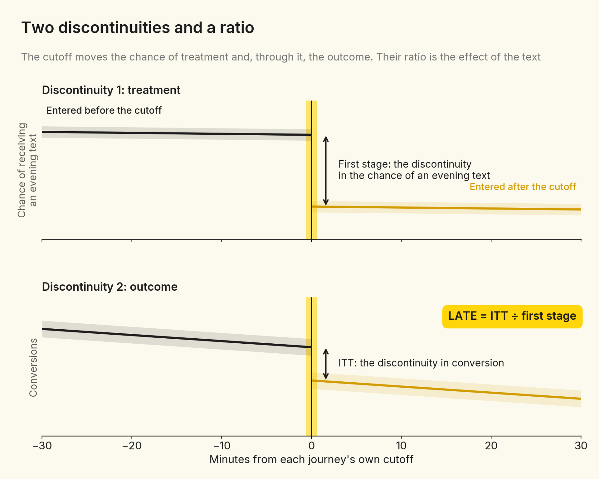
The first discontinuity is in treatment probability across the cutoff, called the first stage, and its size is the share of compliers.
The second discontinuity is in outcomes: the difference in conversion (or opt-out) rates between shoppers just before and just after the cutoff, observed across all shoppers – always-takers, never-takers, and compliers together. This is the intent-to-treat effect, or ITT.
The ITT is real, but diluted. A substantial share of shoppers in the before-cutoff group are always-takers or never-takers, whose treatment the cutoff doesn't change. Their outcomes look the same on both sides, so they add nothing to the discontinuity, but they still count as additional zero effects in the average.
Imagine 1,000 shoppers on each side of the cutoff. Crossing the cutoff takes the evening text away from 500 of them: the compliers. Now suppose the before-cutoff group ends up with ten more purchases than the after-cutoff group. Those ten purchases can't come from the 500 shoppers whose treatment didn't change, so they must come from the 500 compliers. Among the shoppers the cutoff actually affects, receiving the text raises the chance of purchase by 10 in 500, or two percentage points. That's twice as large as the one-point gap between the two crowds, because the gap was being spread over everyone – including those who did not experience any incremental effect.
The local average treatment effect (LATE) corrects this dilution by dividing the ITT by the share of compliers, the first stage:

The word “local” means that this effect applies to compliers at the cutoff, not to every shopper near it.
A natural experiment is only as credible as its assumptions – we need to check them before trusting any estimate.
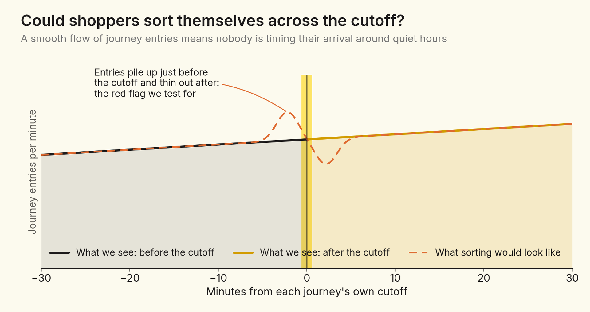
If shoppers, or some system acting on their behalf, could time their journey entry around the cutoff, the two sides would stop being comparable. The sign would be bunching: unusually many entries just on one side of the cutoff and unusually few on the other. This is what a density test looks for. We see millions of journey entries on each side, flowing smoothly across the cutoff minute, just as you'd expect when shoppers have no idea when quiet hours begin.
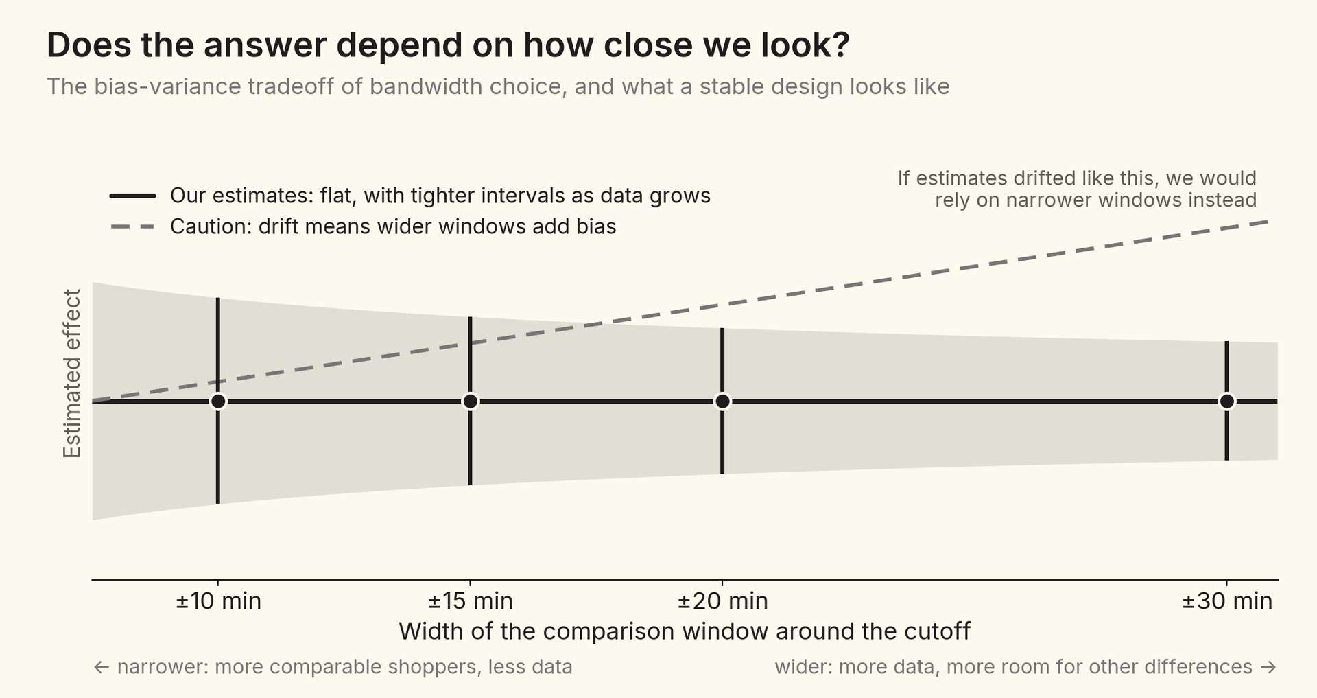
Every RDD faces a choice of the width of the window around the cutoff – the bandwidth. A narrow window compares the most similar shoppers but uses less data. A wide window uses more data but asks us to believe that shoppers further apart in time are still comparable. It's a classic bias-variance tradeoff.
We estimate everything at four bandwidths: ±10, ±15, ±20, and ±30 minutes. If the comparison were contaminated by something that changes over the evening, such as a different mix of shoppers or other sends firing nearby, estimates would drift as the window widened. They don't. Both the first stage and the effects stay flat, while confidence intervals tighten as we add data. That lets us use the widest window for any follow-up analysis with higher granularity.
A regression discontinuity buys credibility by being very local to the quiet-hours cutoff, but can we learn anything about the shoppers throughout the rest of the day?
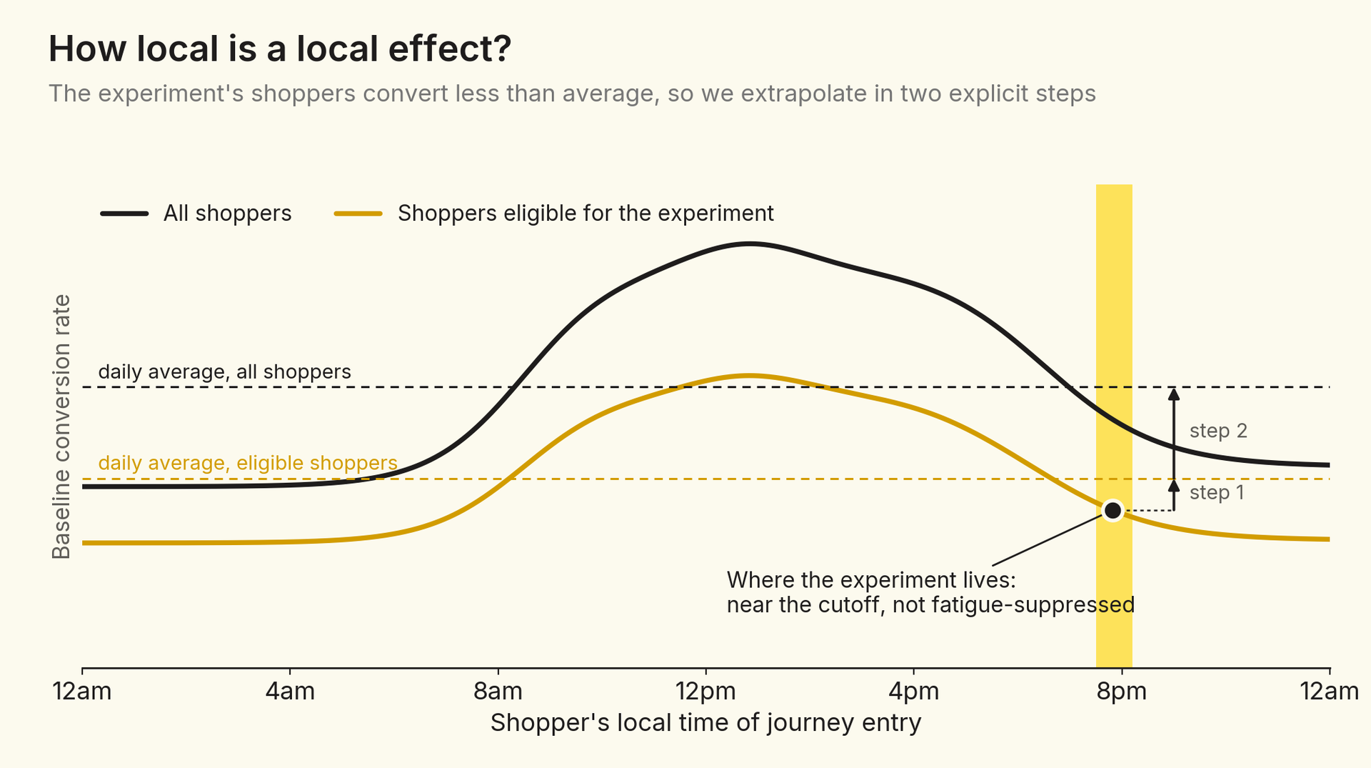
Two features make the experiment's population different from the average shopper. First, it lives in the evening, around the start of quiet hours, when baseline conversion is lower than at midday. Second, it excludes shoppers whose journey messages were blocked by fatigue rules, typically shoppers who received other journeys earlier in the day and may already have converted or opted out.
As a result, the RDD estimate is likely a conservative floor. One way to extrapolate beyond it is to assume that the incremental effect scales in proportion to the baseline conversion and opt-out rates, and then to adjust for the population difference in two steps (see Figure 7):
The intuition is that a message works like a multiplicative nudge: a shopper who is twice as likely to buy anyway is assumed to be twice as responsive to the reminder. That's a reasonable assumption, but it is an assumption rather than a finding. At Attentive, we use a range, from the conservative baseline to the more aggressive extrapolated values, rather than a single number.
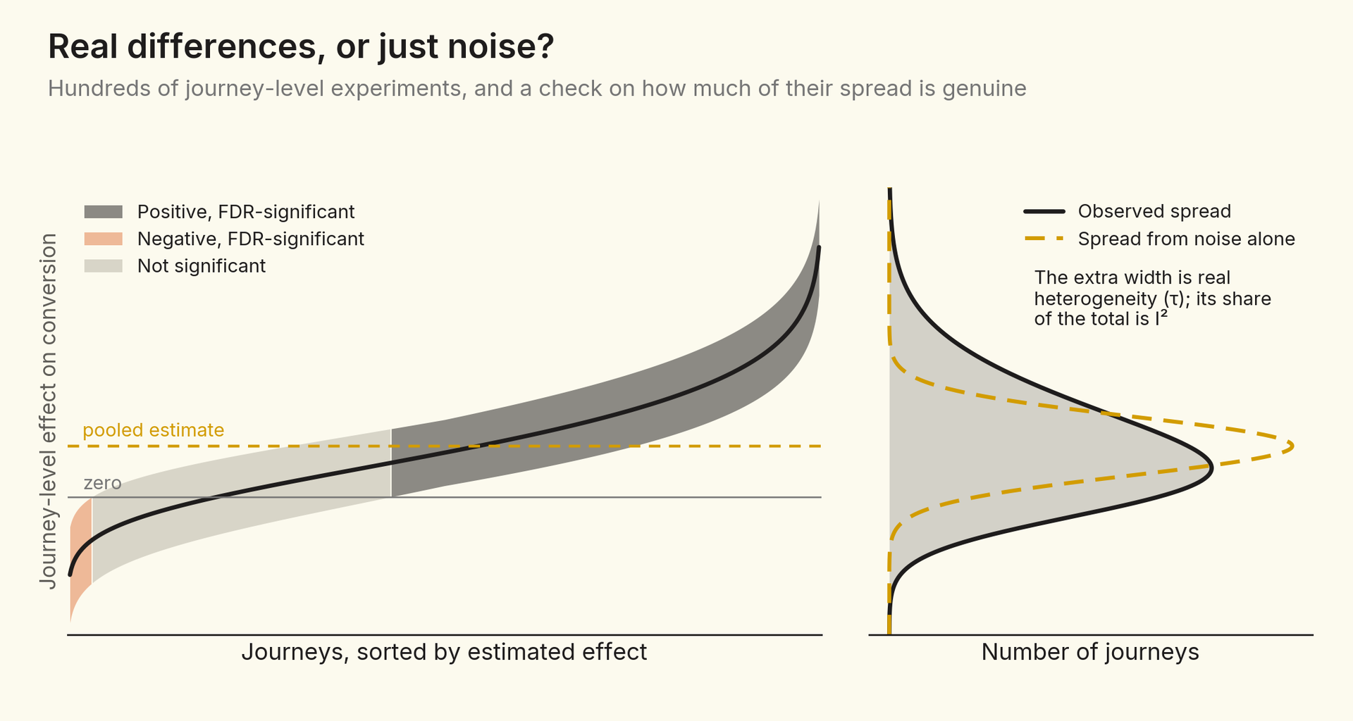
Because every journey has its own cutoff, every journey is its own small natural experiment. To learn the incremental performance of a particular journey, we estimate a saturated regression with a separate fixed effect for each journey. That gives every journey its own first stage and its own ITT, and their ratio is a LATE estimate for every journey.
Because we estimate hundreds of journey-level effects at once, we account for multiple hypothesis testing when constructing confidence intervals and judging significance, so that no journey looks significant simply by chance. We also separate the sampling-noise component of the observed variation across journeys from genuine differences in their effects, which tells us how much of the variation is real.
Once we know journeys genuinely differ, we can ask what the high-lift (low-opt-out) journeys have in common. To answer, we regress each journey's estimated effect on journey and audience characteristics.3
An important caveat sits underneath this analysis. Each journey's effect is causal, because it comes from the natural experiment. But the explanation of why some journeys have larger effects is correlational. Features like offer exposure or send delay weren't randomly assigned across journeys, so the regression tells us which characteristics travel with higher incrementality, not that changing one would necessarily raise it. Its job is to generate well-founded hypotheses for the next round of experiments.
Measuring incrementality usually means choosing between credibility and cost. Randomized holdouts are credible but expensive; attribution is cheap but often answers a different question. A fuzzy RDD design offers a third path where we can get credible incremental estimates for conversions and opt-outs at large scale, but at the cost of finding the right rule in our data and understanding the local nature of our findings.
Quiet hours turned out to be such a rule: a send-time cutoff provides a comparison of otherwise identical shoppers – an incremental contrast. Because every journey has its own cutoff, the same design produced not one experiment but hundreds, enough to study who responds and why.
Most products are full of rules like this one: eligibility thresholds, send windows, frequency caps, rollout dates. Each is a potential natural experiment. The work lies in recognizing them, checking that they behave like experiments, and being precise about which question each one allows us to answer.


