

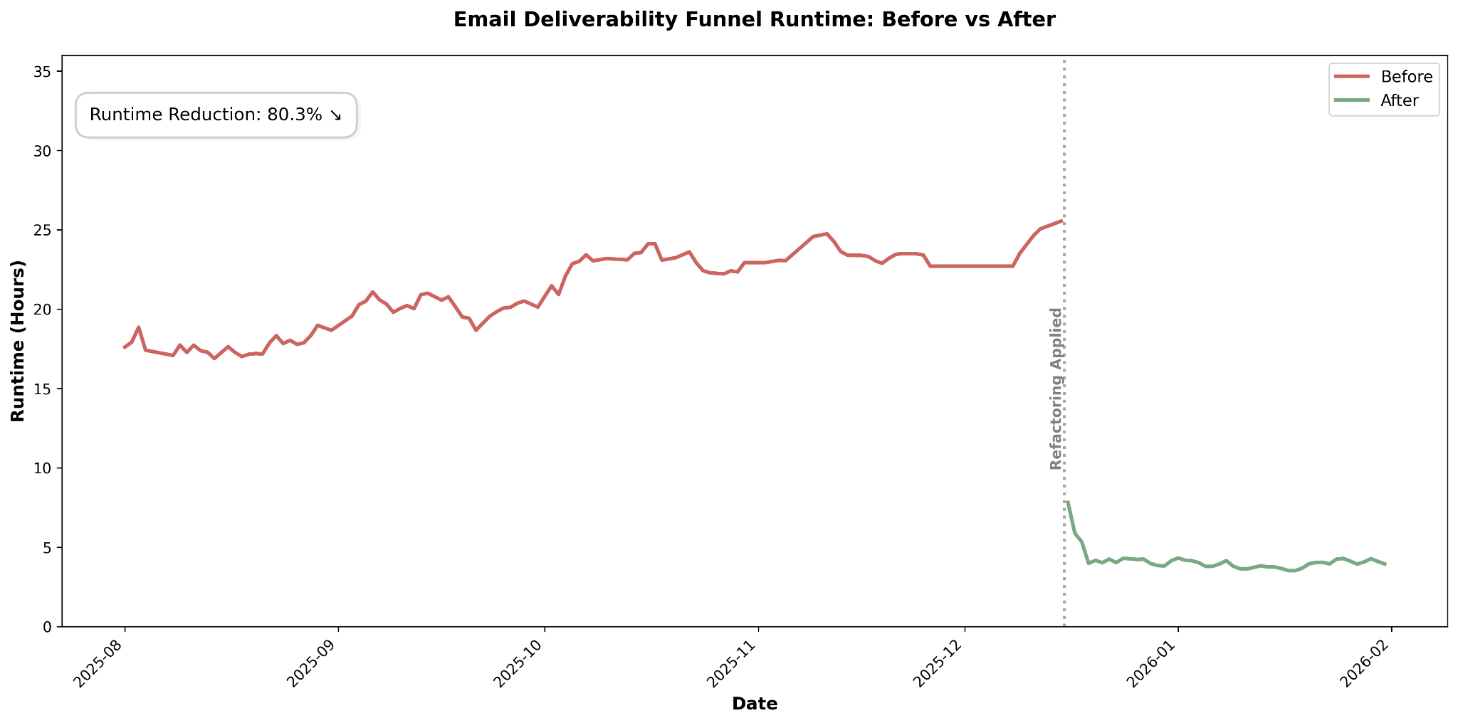
In this article, we share how we cut the runtime of one of our largest volume snowflake DBT models from 26 hours down to just 4. The refactoring approach required us to apply some unusual, but interesting methods (array columns, delta table) to ensure that we aggregated the data accurately and efficiently despite an unbounded historical lookback period for incoming events.
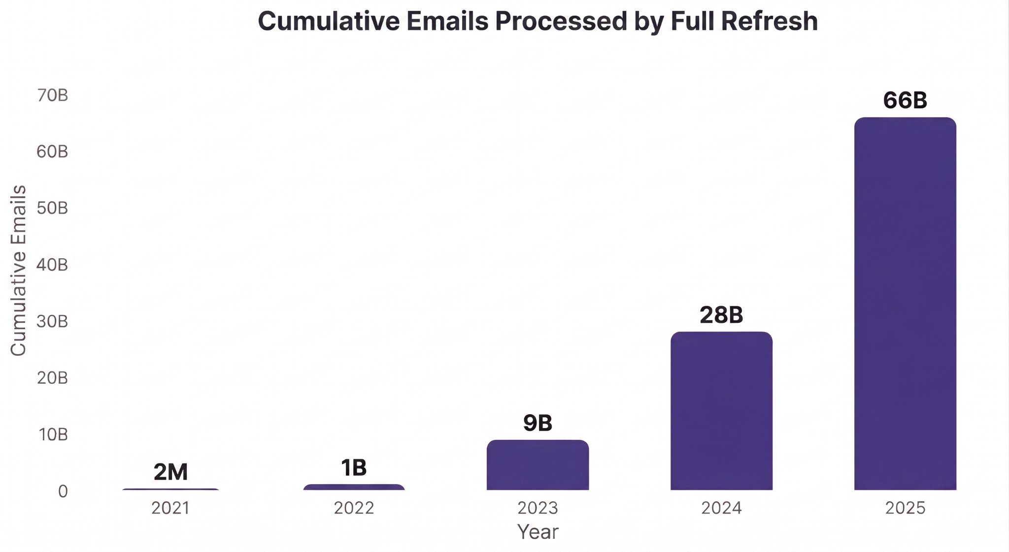
Email is one of Attentive’s rapidly growing messaging channels for marketing communications. In 2025 alone, Attentive’s clients sent over 35 billion emails to their customers, more than double the amount sent the year prior and projected to double again in 2026 at the time of this writing.
Within the world of email, email deliverability is an essential signal that enables marketers to view the lifecycle of an email, from sending the email to landing in a customer’s inbox.
Understanding deliverability means understanding whether or not your emails are being seen by customers and generating revenue.
In Attentive’s internal Snowflake data warehouse, one core DBT model powers our email deliverability analytics: email_delivery_funnel_stats.
The rapid growth of the email channel is great for the business, but presents scalability challenges on the engineering side.
When email_delivery_funnel_stats was first created in 2021, the Snowflake DBT model was able to process all-time data within an hour.
By 2025, the runtime had exploded to over 26 hours.
And to make matters worse, we had received new use cases requiring that this data be refreshed every 15 minutes (we later negotiated this to every 4 hours) to support same-day deliverability troubleshooting.
It was up to the Business Intelligence Engineering team to drastically cut down the pipeline’s runtime.
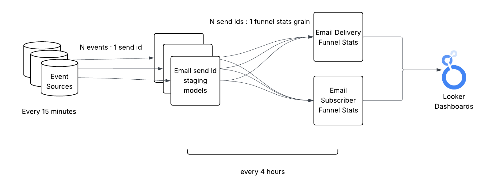
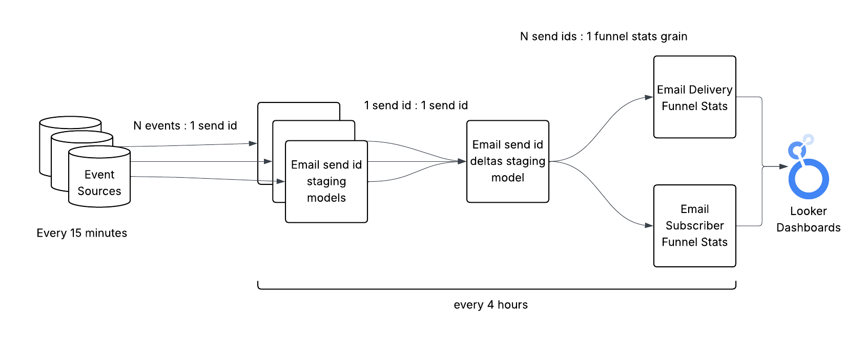
At a high level, the flow of data from event sources to the data consumers is relatively straight forward:
email_delivery_funnel_stats reads from the staging model and event sources and aggregates the data into the final consumer-ready schema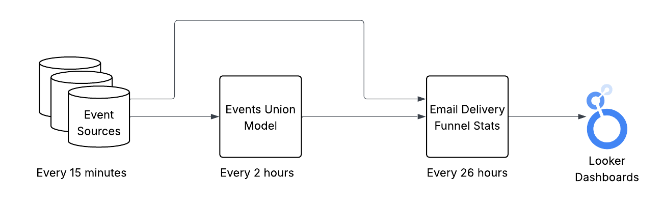
Adding up the runtimes of each step, we can see that the end-to-end latency between the event taking place in reality and appearing in the dashboards can range anywhere from 28-56 hours. Note: only the data available once the model begins will be processed. Data arriving while the model is running will have to wait for the next time the model runs.
Of the two models our team owns, it’s clear that email_delivery_funnel_stats is the primary runtime bottleneck of the pipeline.
Conceptually, the intent of this model is to match events in the email lifecycle (i.e. sent, delivered, click, conversion) with their corresponding send date and aggregate the events into count metrics. We do this by leveraging each event’s email send ID which links them back to a specific email send.
For example, given these set of events:
Event Sources (in consolidated form for convenience)
We would see these aggregated metrics in the email_delivery_funnel_stats table:
Email Delivery Funnel Stats
The grain of this table is a combination of several key attributes shared between many events, such as client id, send date, email domains, and user region.
The main takeaway is that each event has to be matched with the email’s original send date regardless of how far back in the past that send took place. A click in April could be attributed to a send from March. This unbounded lookback for new events makes incremental processing extremely difficult because we have to scan through most of our source and destination data to find the right match on every update.
For this reason, email_delivery_funnel_stats was initially created as a full refresh model, reprocessing all events in all of history and matching them to their corresponding email send event.
This was fine in the beginning when the model finished within an hour, but became unsustainable with a large data volume. We needed a different approach.
Thinking about this pipeline from first principles, we essentially had a process that consumed a set of immutable, append-only data sources and transformed the data into our final aggregated data product.
If we could incrementalize the pipeline to limit the scope of its processing to newly generated events, that should have a big impact on cutting down the runtime just considering the exponentially growing volume of historical data that we were unnecessarily processing on each full refresh.
To confirm that the data volume is the bottleneck (as opposed to query complexity), we looked at the Snowflake query profile for the model. In one sample run, we saw that most of the model runtime was spent performing an aggregation immediately after a source table scan.
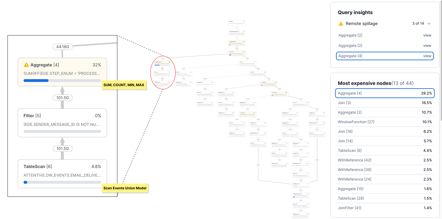
In Snowflake, there is very little that can be done to optimize a simple aggregation of numeric values. We had no choice but to scan through and process every record provided to the aggregation in at best O(N) time complexity.
The only choice that we had was to either scale up our Snowflake warehouse (expensive and not scaleable) or figure out a way to pass fewer records to the aggregation by incrementalizing the model.
For these reasons, we decided incrementalizing the pipeline would be our core strategy to cut the end-to-end runtime down to 4 hours.
A second important consideration we had for refactoring the model was to improve the long-term maintainability of the pipeline.
The code in email_delivery_funnel_stats, although only 153 lines of SQL, had some room for improvement:
To address these issues, we decided to break out some of the email_delivery_funnel_stats logic into multiple smaller models in a more modular architecture. Each of these models would materialize the intermediate state of the data in a more granular form, eventually aggregating into the final grain in email_delivery_funnel_stats.
We predicted that materializing the data in its more granular intermediate form would:
This all sounded good in theory, but as we soon found out, the implementation was not so simple.
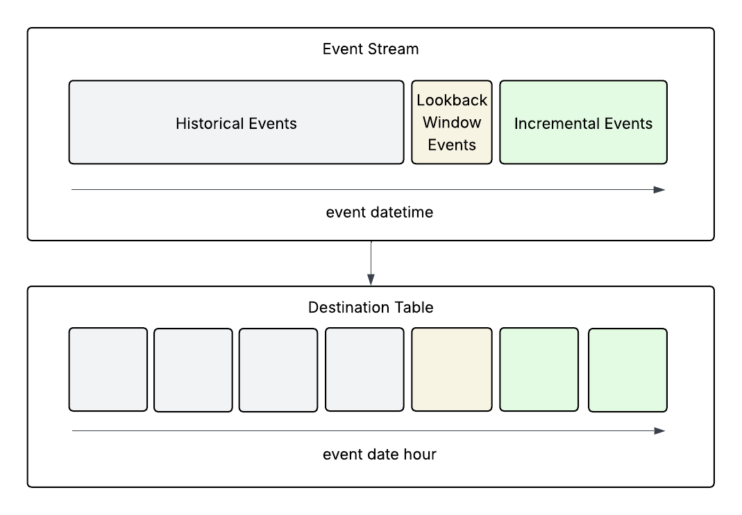
In a typical incremental batch pipeline that consumes from an event stream, events are aggregated by some event datetime grain (i.e. hour, day, month) in the destination table. To handle late arriving events, a lookback window is usually applied as well which reprocesses a small portion of data from the last processed interval.
This pattern works for most pipelines, but not in our case.
In the email deliverability pipeline, we were essentially shuffling the order of the data from event datetime to email send date (via the send id), which cannot be determined without scanning all previous events. This was an unavoidable artifact that was at the core of the value provided by the email_delivery_funnel_stats dataset.
Essentially, we had a dataset that behaves closer to a dimensional model as opposed to a fact table. In other words, the data keeps changing.

The problem with matching events to their send date lies with the lookback window.
Since we were aggregating events by send date, it was not guaranteed that all events linked to a send date grain would be included in the incremental records (other relevant events may have happened in the distant past). So we couldn’t simply aggregate the new records and overwrite the data in the table.
We also couldn't simply add to the existing count without risking double counting events that were processed previously, but were recaptured in the lookback window.
To better illustrate this point, here’s an example of what could happen if we apply a simple lookback window when counting email opens:
In the open events table, we have:
Email Open Events
We load events w and x into the staging table at 2026-01-05 00:01:00:
Email Send ID Opens Staging Model
We process events y and x (again) at 2026-01-05 04:01:00 in the next run since the event falls within our lookback window of 1 hour (1 hour before 2026-01-05 00:01:00):
Email Send ID Opens Staging Model
In this example, we can either:
None of these options looked very appealing, but what if there was a way of knowing which events had already been counted?
Fortunately for us, Snowflake supports array types! This allowed us to store the event uuids which have already been consumed for each send ID.
We used this array to perform an anti-join with the incremental events to exclude any previously processed event. In practice, we left joined and added all incoming events to the existing array then used array_distinct for better performance, but it’s conceptually the same idea.
Here’s the same example from earlier, but with the arrays included:
In the event table, we have:
Email Open Events
We load the data into the staging table at 2026-01-05 00:01:00:
Email Send ID Opens Staging Model
We process the event again at 2026-01-05 04:01:00 in the next run since the event falls within our lookback window of 1 hour:
Email Send ID Opens Staging Model
Now that we can see that event uuid x is already in the array, we can exclude it from being added to the existing opens count. Or just use the array size as the open count.
After we implemented this approach, we had a robust process in place that accurately counted events at the send ID grain.
Unfortunately for us, separating out most of the logic into staging models and incrementalizing every model was not sufficient to bring the total runtime below 4 hours. We still had a bulk of the runtime tied up in the final model which aggregated the send IDs into the final grain (about 8 hours of runtime in that model alone).
Our naive initial approach to incrementalizing the final email_delivery_funnel_stats model looked something like this:
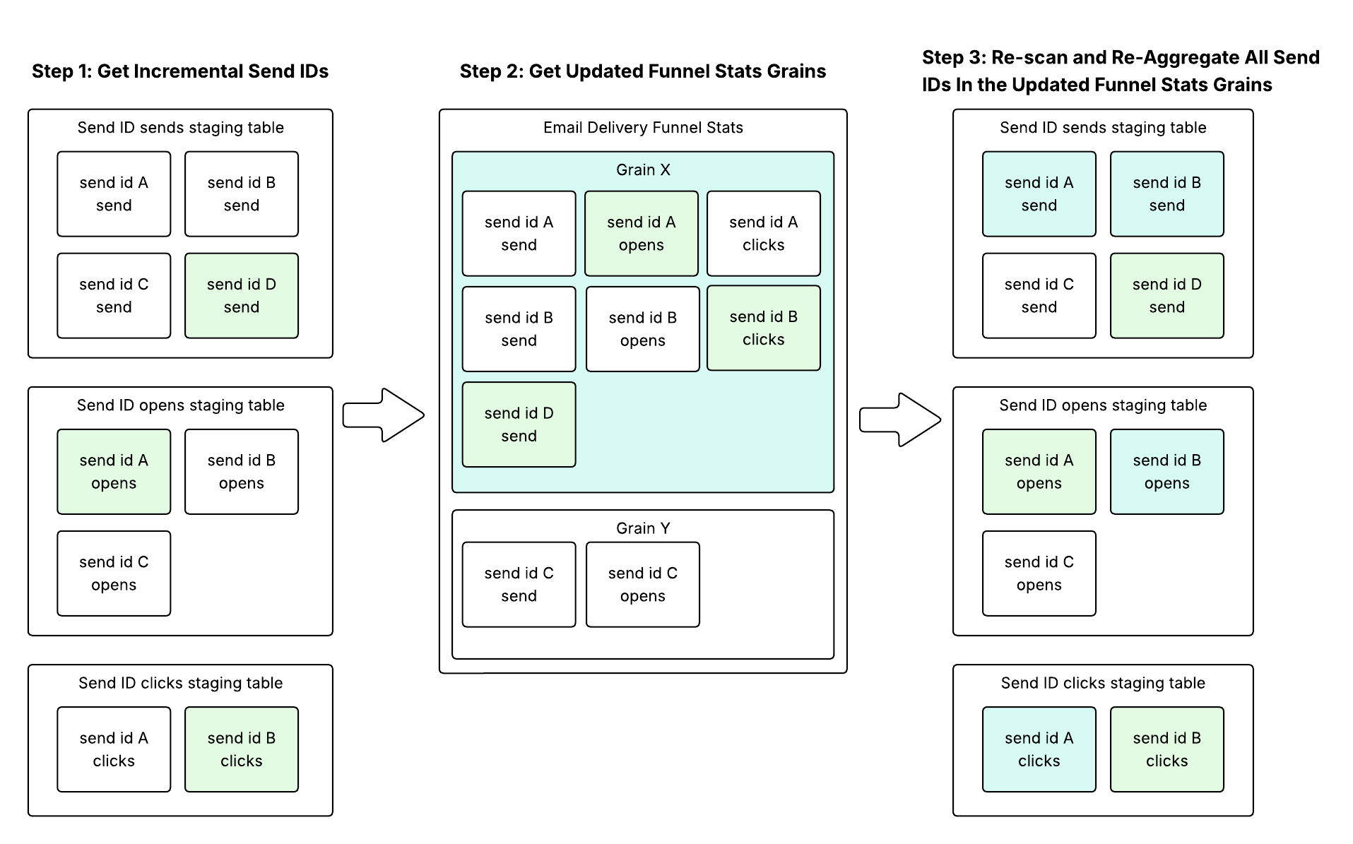
This approach was previously implemented successfully in other pipelines which computed metrics by event date.
However, the problem with this approach was that it could be very inefficient for funnel stats grains that aggregated many send IDs. Although there could be a small number of incremental send ID updates, there was a significant amplification factor that took place between steps 2 and 3.
For example, if funnel stats grain X contained the aggregation of 500,000 send IDs, a single click event coming from a user can trigger a re-aggregation of all 500,000 send IDs, even if most activity for the grain has stopped.
If we were to imitate the send ID staging model logic but with send IDs instead of event uuids, it would not be possible to accurately calculate the funnel stats aggregate amount given a send ID aggregate update. For example:
Current state of the tables:
Email Send ID Clicks Staging Model
Email Delivery Funnel Stats
If we were to receive another click for send ID A, the tables would then look like this:
Email Send ID Clicks Staging Model
Email Delivery Funnel Stats
In this case, we cannot simply add the send ID clicks to the funnel stats clicks, yet at the same time we cannot determine how many of the existing clicks should be subtracted to avoid double counting. With this schema, we are forced to perform a full reaggregation of the entire grain to get an accurate count.
Although this approach didn’t quite work as is, it did hint at the solution to this problem.
To utilize the existing funnel stats aggregates in our processing, we needed to store information which would allow us to determine exactly how much of the send ID aggregates to add to the funnel stats aggregates while excluding what had already been counted.
We can express the solution to this problem with an equation that derives the correct aggregation for each funnel stats grain as follows:

In other words, we just needed to add up the deltas between the new aggregates and the old aggregates for each send ID to the old funnel stats aggregate to derive the new funnel stats aggregate.
We decided to create a new staging model which would handle joining all the staging send IDs together and storing these new and old aggregate deltas for each send ID.
The schema for the send ID deltas model looked something like this:
And this was how it fit in our pipeline:
If we go back to the previous example, the flow of the data would be as follows:
Current state of the tables:
Email Send ID Clicks Staging Model
Email Send ID Deltas Staging Model
Email Delivery Funnel Stats
If we receive another click for send ID A:
Email Send ID Clicks Staging Model
Email Send ID Deltas Staging Model
Email Delivery Funnel Stats
One tradeoff with this approach though was that the deltas model and any models which consume from it were not idempotent. If the deltas model reran prior to the values being consumed, we needed to ensure that new deltas were added to the existing deltas rather than overwriting them. Similarly, the downstream funnel stats models must consume the deltas exactly once to avoid overcounting.
Fortunately, these were solvable tradeoffs and well worth the performance gains we saw from this approach. We implemented guard rails in DBT to compare last updated timestamps between the deltas and funnel stats models to either add to/overwrite the deltas or consume/not consume the deltas.
By implementing this delta table, we now had an efficient way of accurately calculating the funnel stats aggregates in an incremental fashion.
After refactoring the pipeline, we achieved a consistent runtime right within the 3-4 hour range!
According to our key stakeholders, the messaging operations team, the runtime benefits were "enormous" in terms of their ability to support customers. With a much faster refresh cadence, the new pipeline empowered them to perform on-demand deliverability troubleshooting for our clients with fresher data.
There were a few other interesting challenges in this project that we didn’t have time to cover here, but if these types of technical challenges excite you, let’s get in touch!


