


Personalization at scale is hard. To champion Attentive’s thousands of brands, we strive to provide deeply personalized experiences for every online shopper. In this post, I’ll walk through how we scaled our product recommendation system from thousands to hundreds of thousands of users per second, while simultaneously reducing cost and complexity. After extensive evaluation and frustrating attempts to optimize off-the-shelf solutions, we reached a breakthrough when we stepped back, re-assessed the fundamental computer science algorithmic necessities of the core calculation, and implemented the computation ourselves using LibTorch.
This project reflects how we solve problems here: start simple, challenge assumptions, and balance practical engineering with cutting-edge ML. If you already want to know more, be sure to check out openings on our team.
In a previous blog post, our ML team described the creation of a two-tower model that leverages deep learning to compress rich, high-dimensional behavioral and catalog data into dense vector embeddings. Attentive incorporates the data from thousands of brands, millions of subscribers, and billions of events, allowing us to tailor messages to each individual subscriber from the brands they love. This deep learning architecture allows us to place every subscriber and every product into a shared embedding space. To find the best products for each subscriber, we simply want to find the product embeddings that are most similar to a given subscriber’s embedding. Mathematically, we can describe this as maximizing the cosine similarity between the vector embeddings.
In our first production release, we sidestepped the serving complexity by precomputing the top 100 recommendations per user. This worked reasonably well for messages where the entire product catalog is in-scope, but falls short when we consider dynamic catalogs. In particular, product filters are challenging. For example, if a clothing brand wants to highlight their latest jeans, then applying those product filters might exclude all the precomputed recommendations for a given subscriber if they’ve only ever purchased shirts and shoes. Even for unfiltered campaigns, we also want to respect real-time changes to inventory status (we never send recommendations promoting out-of-stock products). For truly personalized marketing, we needed to compute recommendations at send time.
Our First Attempt: PGVector (Promising but Costly)
We began this project using PGVector, a developer-friendly PostgreSQL extension that natively supports vector search. For example, you can order results by cosine distance like this:
SELECT *
FROM products p
JOIN subscribers s ON (p.company_id = s.company_id)
WHERE s.id = 12345
ORDER BY p.embedding <=> u.embedding DESC
LIMIT 5;
That `<=>` operator does the heavy lifting: it computes the cosine distance between the vectors, sorts the results accordingly, returning the top five. It’s a simple and easy implementation that fits in well with the rest of our product catalog systems, which are already built around a PostgreSQL database. We quickly built a proof-of-concept and were delighted by the initial results.
That excitement, however, faded during load testing. To operate at Attentive’s scale, we need to support peak loads exceeding 50,000 queries per second (QPS). PGVector on AWS RDS delivered roughly 20 QPS per CPU, which meant we’d need a vast fleet of database replicas costing an estimated $50,000 per month just to meet demand. Clearly, this wasn’t sustainable, so we began looking for ways to optimize.
We then explored Aurora, AWS's "serverless" database product, which supports full PostgreSQL compatibility. Our database needs are inherently bursty: we need to support 50k QPS at peak times, but will often have long bouts of idleness. As a serverless solution, we hoped that Aurora could auto-magically scale up when needed and then scale back down. Unfortunately, while Aurora does deliver tunable elastic capacity, the maximum is only slightly better than what's available via a dedicated RDS instance. In our testing, Aurora's performance scaled proportionally to RDS sizes. That is, allocating 128 “Aurora Compute Units” (half the maximum) was comparable to running on a "24xlarge" RDS instance. From this, we suspected that Aurora is running on the same physical hardware as RDS. The so-called "serverless" option provides thin-slicing and rapid scaling, but is ultimately still bound by the same maximum server size.
In our extensive testing of RDS, Aurora, as well as some additional vector database products, we realized that our test setup was actually more demanding than what we really need. As described above, this calculation is equivalent to running the k-nearest-neighbors (kNN) algorithm, which computes the exact distance between the subscriber’s embedding and every product. For recommender systems, it’s sufficient to use approximate-nearest-neighbors (aNN). There are a dizzying plethora of options for aNN algorithms which each have their own performance differences. PGVector supports the Hierarchical Navigable Small World (HNSW) algorithm by way of indexing: we can construct an index in advance and then use it to accelerate query performance (albeit by accepting an accuracy tradeoff based on the amount of approximation). In our tests, this produced about a 3x improvement over exact kNN when searching the entire product catalog. That’s helpful, but still falls short of our expectations. More frustratingly, the HNSW performance advantage disappeared once we introduced product filters, which was the raison d'être for calculating recommendations at send time!
Fortunately, the inefficacy of aNN for filtered queries gave us a clue as to the source of our performance issues.
Most of us learn about algorithmic complexity in school and apply it to toy examples during interviews—but this project reminded me how essential it is in production. PGVector was appealing because it neatly integrated vector search into SQL. We were initially drawn to PGVector because it offered vector distance computation as a black-box abstraction, neatly integrated into SQL. For application developers, that’s appealing—it’s convenient to stand on the shoulders of well-designed tools. But in this case, the abstraction conceals some crucial trade-offs. To reason clearly about performance, we need to dig into the underlying mechanics.
Whether we use k-nearest neighbors (kNN) or approximate nearest neighbors (aNN), computing recommendations requires loading every product embedding and every subscriber embedding into memory.
Either way, the system must eventually read all embeddings from storage. This leads us to an important principle: the Big-Omega (Ω) lower bound on the algorithm’s runtime. No matter how clever or optimized our implementation, the best-case complexity is at least:
Ω(|S| + |P|)
(where |S| = number of subscribers, |P| = number of products)
Once we frame the problem this way, it becomes clear: we want to minimize the number of times we pay this cost. Ideally, we would load all of the embeddings into memory exactly once. But so far, we’ve been querying the database once per user, potentially paying the loading cost |S| times and increasing our worst-case cost to:
O(|S| * (|S| + |P|)
In practice, the database will cache some recent query results and our actual performance will be somewhere between the Big-Omega and Big-O bounds, depending on what other queries are hitting the database.
Fortunately, our 50k QPS performance target is largely driven by the needs of marketing campaigns, which have an inherently predictable access pattern. We never send a campaign to 1 subscriber. Typical campaigns target hundreds of thousands or even millions of subscribers, all from the same brand, using the same product catalog. That access pattern lets us rethink our algorithm. The ideal approach looks like this:
This structure minimizes the number of full catalog loads and lets us scale more predictably.
It also highlights why aNN methods are ineffective in our filtered setting. While aNN improves query-time complexity, it introduces index-build time costs. Creating the index still requires scanning every product embedding. And if a campaign includes filters (e.g., “only shoes under $100”), those filters may invalidate the index. The system either reverts to a sequential scan or builds a new index for the filtered subset. In both cases, we’ve now paid the cost of loading product embeddings twice: once for index creation and again for filtered retrieval. That is less efficient than just using exact kNN.
In summary: while black-box abstractions are convenient, understanding lower bounds, workload characteristics, and access patterns are critical. In this case, thinking in terms of Big-O and Big-Omega helped us identify performance bottlenecks and choose a design that better fits our real-world needs.
Realizing the theoretical best-case performance helped us uncover a subtle but important flaw in how we were framing our goal:
We originally set out to build a system capable of handling 50,000 queries per second. But in practice, that’s not what the system actually needs to achieve. What we really need is the ability to generate recommendations for 50,000 subscribers per second—regardless of how many individual queries that takes.
Once we recognized that campaign traffic is inherently batch-oriented, the solution became much simpler. We don’t need 50,000 independent queries; we need just two:
Armed with this insight, we built a quick proof of concept. We exported a representative sample of embeddings to JSON files and wrote a simple Python script using PyTorch in under 100 lines of code. Running on a spare development box, this script was able to compute personalized recommendations for more than 20,000 subscribers per second. What started as a $50k/month scalability problem now looks like a problem we can solve with three under-used dev boxes.
What makes this implementation so fast is PyTorch’s highly optimized support for matrix math—particularly batched dot products. To understand how this works, let’s take a closer look at cosine similarity. The cosine similarity between two vectors u and v is defined as:
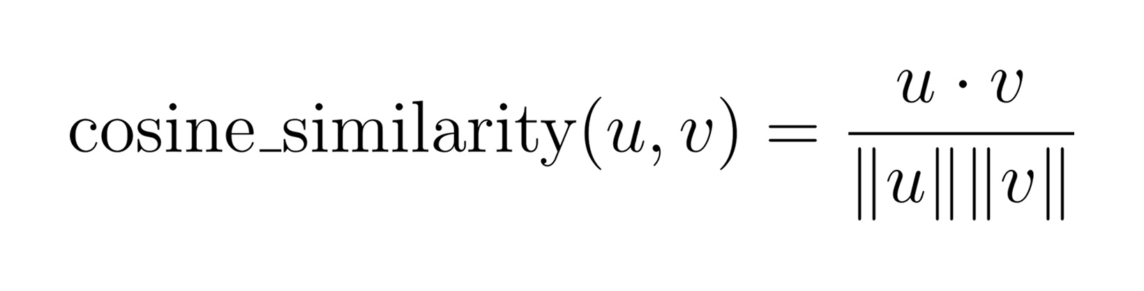
That’s just the dot product of the two vectors, divided by the product of their magnitudes. If we normalize all embeddings in advance (so that |u| = |v| = 1), then the denominator becomes 1 and cosine similarity reduces to:
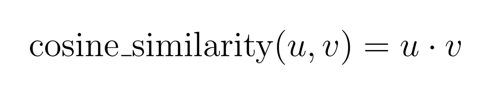
So, computing recommendations becomes a matter of calculating the dot product between each subscriber embedding and each product embedding.
Now suppose we have:
To compute the cosine similarity between every subscriber and every product, we can multiply U by the transpose of P:

Each element is computed as the dot product between the i-th row of U and the j-th row of P:

In other words, matrix multiplication between U and Pᵗ is just a highly optimized way of computing all N × M dot products in parallel.
PyTorch is highly optimized for this kind of operation. Under the hood, it leverages hardware acceleration (e.g., AVX on CPU or CUDA on GPU) to perform these matrix multiplications at extremely high throughput. Even on a laptop CPU, PyTorch can easily perform millions of dot products per second.
This is why our proof-of-concept script, running locally, was able to generate recommendations for over 20,000 subscribers per second—a throughput that far exceeds what we could affordably achieve using database queries alone. By framing the problem in terms of matrix operations rather than individual queries, we unlocked a vastly more efficient and scalable solution.
Having validated this batch-oriented solution with a proof-of-concept, our next step was to build a production-grade solution around the same core insight.
Python and PyTorch were ideal for prototyping and are widely used at Attentive for offline processing (such as training the Two Tower ML model that creates the embeddings). But for transactional workloads, we prefer the reliability and performance benefits of statically typed languages and long-running JVM services deployed in Kubernetes. Fortunately, the optimized vector code leveraged by PyTorch is also available as a C++ distribution (LibTorch), which has java bindings available via the DJL (Deep Java Library) project. DJL offers a nearly one-to-one mapping of the PyTorch API, which makes porting our proof-of-concept trivial. In just a few hours, we had a robust, production-ready Java implementation with the same underlying performance characteristics.
Building a bespoke recommendation workflow gave us flexibility that off-the-shelf vector databases do not. We know the most expensive operation in this process is loading all of the embeddings from disk, so we designed our system to do that at the most opportune time. In particular, we can begin loading product embeddings concurrently with campaign audience selection. Campaigns typically target millions of subscribers and determining the subscriber segment can take several seconds. Rather than wait idly, we use that time to prepare embeddings in memory. This turns existing latency into productive work, allowing us to calculate recommendations at scale without adding meaningful new latency.
This orchestration is powered by Temporal, our preferred framework for managing distributed workflows. Once both subscriber and product embeddings are in memory, the recommendation calculation becomes embarrassingly parallelizable: each subscriber’s top-k product list can be computed independently. Using Temporal, we split the workload into mini-batches and enqueue them. A pool of workers (each running our Java/DJL implementation) then picks up and processes these batches in parallel. This architecture enables us to horizontally scale the most computationally expensive part of the pipeline by simply adding more worker nodes.
The result is a system that meets our demanding throughput requirements, scales elastically during workload spikes, and remains cost-efficient—thanks to a deep understanding of the underlying algorithms and intentional control over when and how expensive operations are performed.
After implementation, our final task was to run a series of demanding load tests to ensure everything performed as expected and to surface any remaining bottlenecks.
The results dramatically exceeded our goal: with just 32 worker nodes, we achieved nearly 800,000 users-per-second. That’s a 16x improvement over our original goal of 50k.
For Attentive, that means our recommendation engine won’t crumble on Black Friday, and engineers can sleep at night knowing we’ve built something robust.
The takeaway here is simple: when the obvious tool (aNN) fails, don’t be afraid to flip the problem on its head. If you’re a creative thinker who isn’t afraid to take risks and tackle dynamic challenges like this one, let’s talk– our team is growing!


